
You are here: Start » Deep Learning
Deep Learning
Table of contents:
- Introduction
- Anomaly Detection
- Feature Detection
- Object Classification
- Instance Segmentation (deprecated)
- Point Location
- Object Location
- Reading Characters
- Locating Text
- Troubleshooting
1. Introduction
Deep Learning is a breakthrough machine learning technique in computer vision. It learns from training images provided by the user and can automatically generate solutions for a wide range of image analysis applications. Its key advantage, however, is that it is able to solve many of the applications which have been too difficult for traditional, rule-based algorithms of the past. Most notably, these include inspections of objects with high variability of shape or appearance, such organic products, highly textured surfaces or natural outdoor scenes. What is more, when using ready-made products, such as our FabImage Deep Learning, the required programming effort is reduced almost to zero. On the other hand, deep learning is shifting the focus to working with data, taking care of high quality image annotations and experimenting with training parameters – these elements actually tend to take most of the application development time these days.
Typical applications are:
- detection of surface and shape defects (e.g. cracks, deformations, discoloration),
- detecting unusual or unexpected samples (e.g. missing, broken or low-quality parts),
- identification of objects or images with respect to predefined classes (i.e. sorting machines),
- location, segmentation and classification of multiple objects within an image (i.e. bin picking),
- product quality analysis (including fruits, plants, wood and other organic products),
- location and classification of key points, characteristic regions and small objects,
- optical character recognition.
The use of deep learning functionality includes two stages:
- Training – generating a model based on features learned from training samples,
- Inference – applying the model on new images in order to perform the actual machine vision task.
The difference to the traditional image analysis approach is presented in the diagrams below:
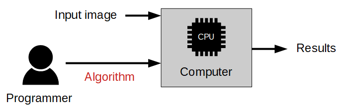
Traditional approach: The algorithm must be designed by a human specialist.
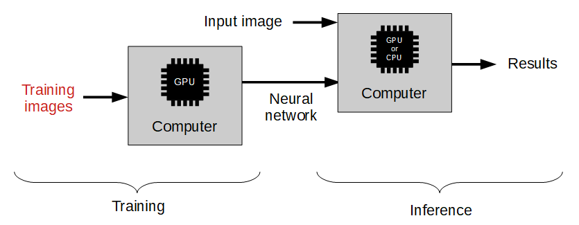
Machine learning approach: We only need to provide a training set of labeled images.
Overview of Deep Learning Tools
- Anomaly Detection – this technique is used to detect anomalous (unusual or unexpected) samples. It only needs a set of fault-free samples to learn the model of normal appearance. Optionally, several faulty samples can be added to better define the threshold of tolerable variations. This tool is useful especially in cases where it is difficult to specify all possible types of defects or where negative samples are simply not available. The output of this tool are: a classification result (normal or faulty), an abnormality score and a (rough) heatmap of anomalies in the image.
- Feature Detection (segmentation) – this technique is used to precisely segment one or more classes of pixel-wise features within an image. The pixels belonging to each class must be marked by the user in the training step. The result of this technique is an array of probability maps for every class.
- Object Classification – this technique is used to identify an object in a selected region with one of user-defined classes. First, it is necessary to provide a training set of labeled images. The result of this technique is: the name of detected class and a classification confidence level.
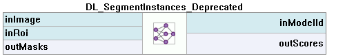
- Instance Segmentation (deprecated) – this technique is used to locate, segment and classify one or multiple objects within an image. The training requires the user to draw regions corresponding to objects in an image and assign them to classes. The result is a list of detected objects – with their bounding boxes, masks (segmented regions), class IDs, names and membership probabilities.
- Point Location – this technique is used to precisely locate and classify key points, characteristic parts and small objects within an image. The training requires the user to mark points of appropriate classes on the training images. The result is a list of predicted point locations with corresponding class predictions and confidence scores.
- Reading Characters – this technique is used to locate and recognize characters within an image. The result is a list of found characters.
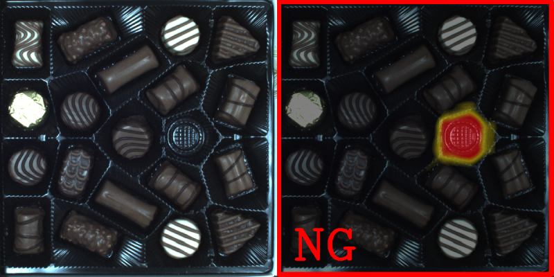
An example of a missing object detection using FisFilter_DL_DetectAnomalies2 tool.
Left: The original
image with a missing element. Right: The classification result with a heatmap of anomalies.
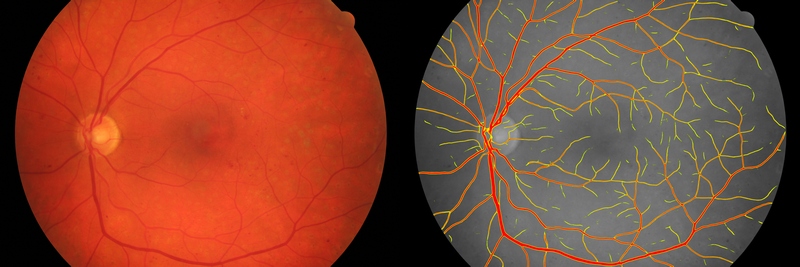
An example of image segmentation using FisFilter_DL_DetectFeatures tool.
Left: The original
image of the fundus. Right: The segmentation of blood vessels.
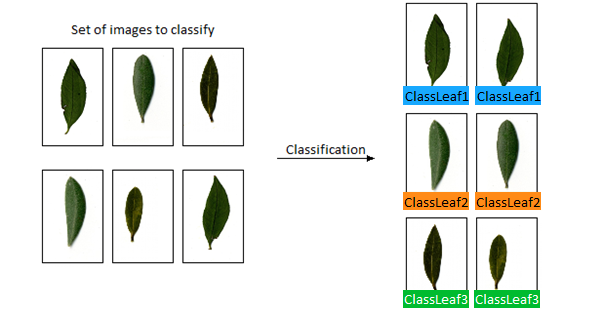
An example of object classification using FisFilter_DL_ClassifyObject tool.
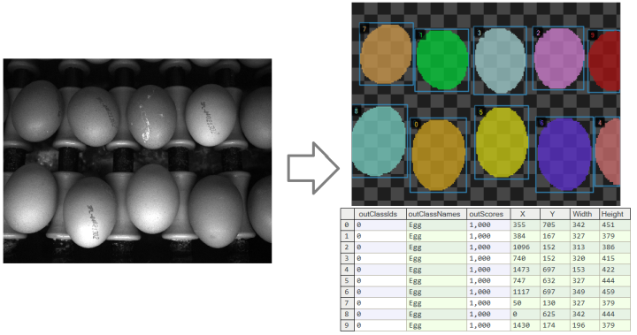
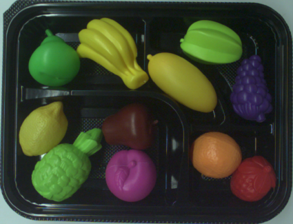
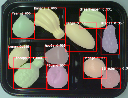
An example of instance segmentation using FisFilter_DL_SegmentInstances_Deprecated tool. Left: The original image. Right: The resulting list of detected objects.
The Instance Segmentation model is trainable in 5.3 and older versions only. In more recent releases, models trained in 5.3 and older versions can only be inferred.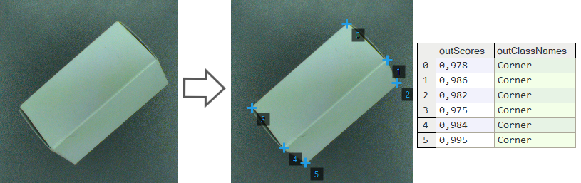
An example of point location using FisFilter_DL_LocatePoints tool. Left: The original image. Right: The resulting list of detected points.
An example of optical character recognition using FisFilter_DL_ReadCharacters tool. Left: The original image. Right: The image with the recognized characters drawn.
Basic Terminology
You do not need to have the specialistic scientific knowledge to develop your deep learning solutions. However, it is highly recommended to understand the basic terminology and principles behind the process.
Deep neural networks
FabImage provides access to several standardized deep neural networks architectures created, adjusted and tested to solve industrial machine vision tasks. Each of the networks is a set of trainable convolutional filters and neural connections which can model complex transformations of an image with the goal to extract relevant features and use them to solve a particular problem. However, these networks are useless without proper amount of good quality data provided for training process. This documentation presents necessary practical hints on creating an effective deep learning model.
Depth of a neural network
Due to various levels of task complexity and different expected execution times, the users can choose one of five available network depths. The Network Depth parameter is an abstract value defining the memory capacity of a neural network (i.e. the number of layers and filters) and the ability to solve more complex problems. The list below gives hints about selecting the proper depth for a task characteristics and conditions.
-
Low depth (value 1-2)
- A problem is simple to define.
- A problem could be easily solved by a human inspector.
- A short time of execution is required.
- Background and lighting do not change across images.
- Well-positioned objects and good quality of images.
-
Standard depth (default, value 3)
- Suitable for a majority of applications without any special conditions.
- A modern CUDA-enabled GPU is available.
-
High depth (value 4-5)
- A big amount of training data is available.
- A problem is hard or very complex to define and solve.
- Complicated irregular patterns across images.
- Long training and execution times are not a problem.
- A large amount of GPU RAM (≥4GB) is available.
- Varying background, lighting and/or positioning of objects.
Tip: Test your solution with a lower depth first, and then increase it if needed.
Note: A higher network depth will lead to a significant increase in memory and computational complexity of training and execution.
Data division
While training the model, we use one set of images to estimate the network weights. This set is called training data and should reflect the problem as well as possible (e.g., in the case of object classification, representants for all considered classes should be present in this set).
To be sure that the learned model generalizes well, or in other words can give similar results with newly seen data, we need to prepare validation data, too. This second set should contain a small number of representative images to the learned problem. A rule of a thumb says, that its size should be 10% of the training data set size and have a good representation of all problems (e.g., at least one image for each class in the case of object classification should be present in validation data).
The images loaded to Deep Learning Editor must be assigned to one of those two datasets before training procedure can follow.
When the amount of data is large, one may want to simulate how the trained model will work on images not used during the training (it allows checking the performance accessible during the inference). In such a case, assign images to test data.
Training process
Model training is an iterative process of updating neural network weights based on the training data. One iteration involves some number of steps (determined automatically), each step consists of the following operations:
- selection of a small subset (batch) of training samples,
- calculation of an error measure for these samples,
- updating the weights to achieve lower error for these samples.
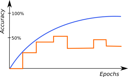
At the end of each iteration, the current model is evaluated on a separate set of validation samples selected before the training process. Depending on the tool, validation set can be automatically chosen from the training samples, or selected by the user. It is used to simulate how neural network would work with real images not used during training. Only the set of network weights corresponding with the best validation score at the end of training is saved as the final solution. Monitoring the training, validation and loss score (blue, orange and purple lines in the figures below) in consecutive iterations gives fundamental information about the progress:
- Training and validation scores are improving and loss score is decreasing – keep training, the model can still improve.
- Training and validation scores has stopped improving and loss score is decreasing – keep training for a few iterations more and stop if there is still no change.
- Loss score is improving – you can stop training, model has probably started overfitting to your training data (remembering exact samples rather than learning rules about features). It may also be caused by too small amount of diverse samples or too low complexity of the problem for a network selected (try lower Network Depth).
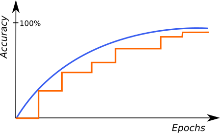
An example of correct training. |
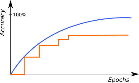
A graph characteristic for network overfitting. |
The above graphs represent training progress in the Deep Learning Editor. The blue line indicates performance on the training samples, the orange line represents performance on the validation samples and the purple line represents the loss function. Please note the blue line is plotted more frequently than the orange line as validation performance is verified only at the end of each iteration.
Stopping Conditions
The user can stop the training manually by clicking the Stop button. Alternatively, it is also possible to set one or more stopping conditions:
- Iteration Count – training will stop after a fixed number of iterations.
- Iterations without Improvement – training will stop when the best validation score was not improved for a given number of iterations.
- Time – training will stop after a given number of minutes has passed.
- Validation Accuracy or Validation Error – training will stop when the validation score reaches a given value.
Preprocessing
To adjust performance to a particular task, the user can apply some additional transformations to the input images before training starts:
- Downsample – reduction of the image size to accelerate training and execution times, at the expense of lower level of details possible to detect. Increasing this parameter by 1 will result in downsampling by the factor of 2 over both image dimension.
- Convert to Grayscale – while working with problems where color does not matter, you can choose to work with monochrome versions of images.
Augmentation
In case when the number of training images can be too small to represent all possible variations of samples, it is recommended to use data augmentations that add artificially modified samples during training. This option will also help avoiding overfitting.
Below is a description of the available augmentations and examples of the corresponding transformations:
- Luminance – change brightness of samples by a random percentage (between -ParameterValue and +ParameterValue) of pixel values (0-255). For a given augmentation values, samples as below can be added to the training set.
- Contrast – difference in brightness or color between elements of an image. This parameter enhances the network to recognize details more effectively. It is specified by a single float value that defines the range of contrast adjustments as (-contrast, contrast). These values can range from -50% to 50%, where 0% indicates no change, 50% represents the maximum increase in contrast, and -50% signifies the maximum decrease in contrast. The default setting is 0%. For instance, if a 20% value is chosen, the contrast change applied to an image will be randomly selected from a range of -20% to 20% and incorporated into the training set.
- Brightness – increase the brightness of samples by multiplying pixel values. This parameter is introduced instead of Luminance in some of Deep Learning tools.
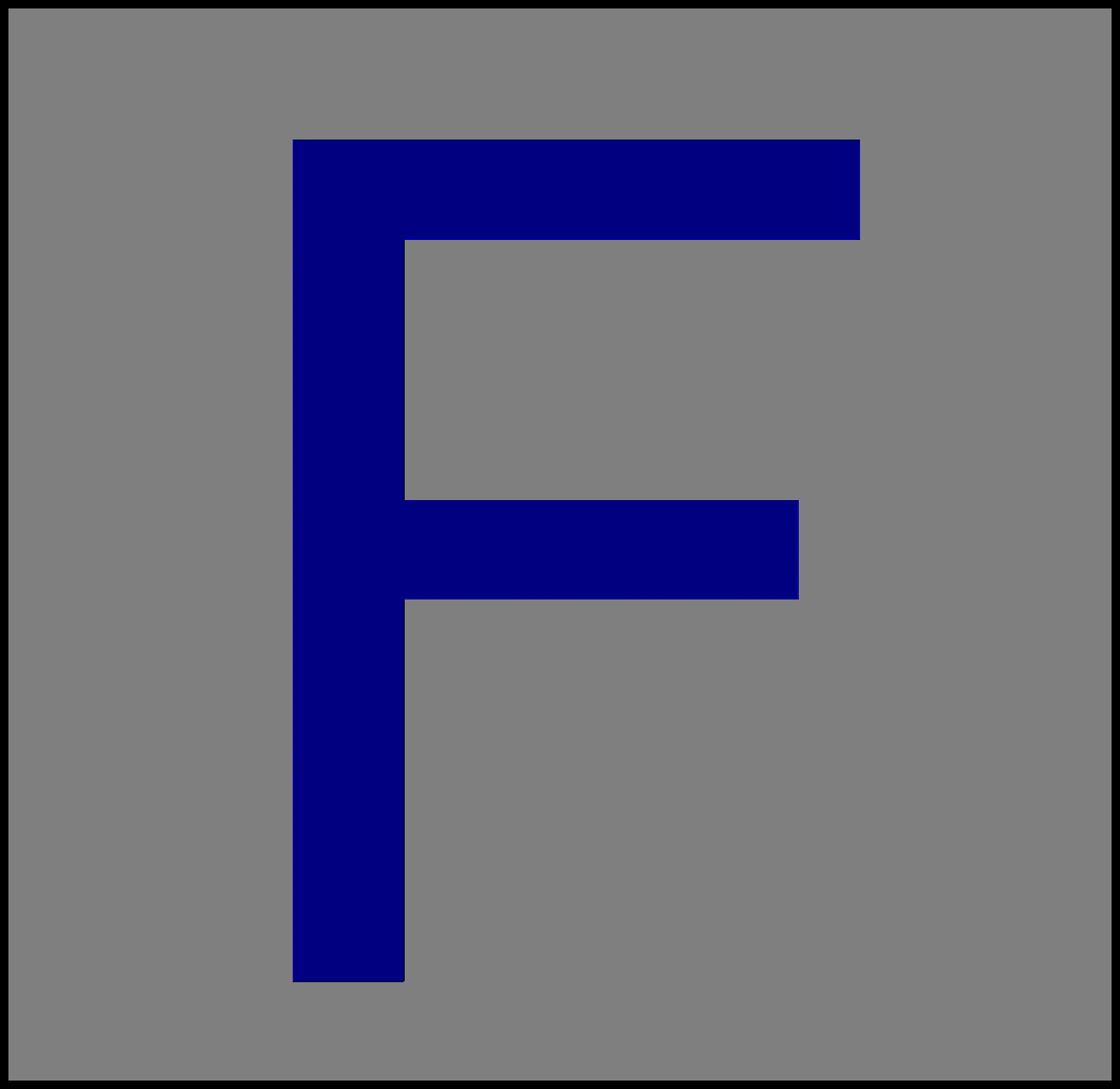
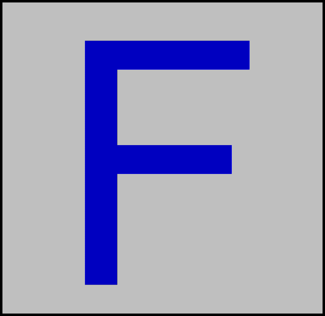
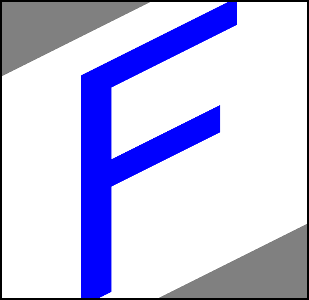
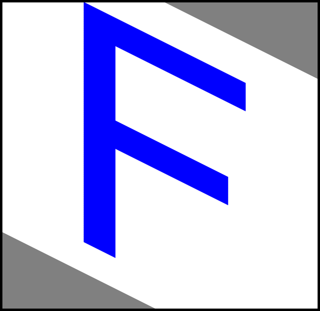
- Noise – modify samples with uniform noise. Value of each channel and pixel is modified separately, by random percentage (between -ParameterValue and +ParameterValue) of pixel values (0-255). Please note that choosing an appropriate augmentation value should depend on the size of the feature in pixels. Larger value will have a much greater impact on small objects than on large objects. For a tile with the feature "F" with the size of 130x130 pixels and a given augmentation values, samples as below can be added to the training set.:
- Gaussian Blur – blur samples with a kernel of a size randomly selected between 0 and the provided maximum kernel size. Please note that choosing an appropriate Gaussian Blur Kernel Size should depend on the size of the feature in pixels. Larger kernel sizes will have a much greater impact on small objects than on large objects. For a tile with the feature "F" with the size of 130x130 pixels and a given augmentation values, samples as below can be added to the training set.:
- Rotation – rotate samples by a random angle between -ParameterValue and +ParameterValue. Measured in degrees.
- Flip Up-Down – reflect samples along the X axis.
- Flip Left-Right – reflect samples along the Y axis.
- Relative Translation – translate samples by a random shift, defined as a percentage (between -ParameterValue and +ParameterValue) of the tile. Works independently in both X and Y dimensions.
- Scale – resize samples relatively to their original size by a random percentage between the provided minimum scale and maximum scale.
- Horizontal Shear – shear samples horizontally by an angle between -ParameterValue and +ParameterValue. Measured in degrees.
- Vertical Shear – analogous to Horizontal Shear.
Luminance=-50. |
Luminance=-25. |
Original image. |

Luminance=25. |

Luminance=50. |

Contrast=-50%. |

Contrast=-20%. |

Original image (0%). |

Contrast=20%. |

Contrast=50%. |
|
Brightness=0.2. |
Brightness=0.5. |
Original image. |
Brightness=1.5. |
Brightness=1.8. |

Original grayscale image. |

Grayscale image. Noise=4. |

Grayscale image. Noise=10. |

Grayscale image. Noise=25. |
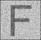
Grayscale image. Noise=50. |
Original RGB image. |
RGB image. Noise=4. |

RGB image. Noise=10. |

RGB image. Noise=25. |
RGB image. Noise=50. |
|
Original image. |

Gaussian Blur=5. |

Gaussian Blur=10. |

Gaussian Blur=25. |

Gaussian Blur=50. |
In Detect Features, Locate Points and Detect Anomalies, for a tile with the feature "F" and given augmentation values, samples as below can be added to the training set.
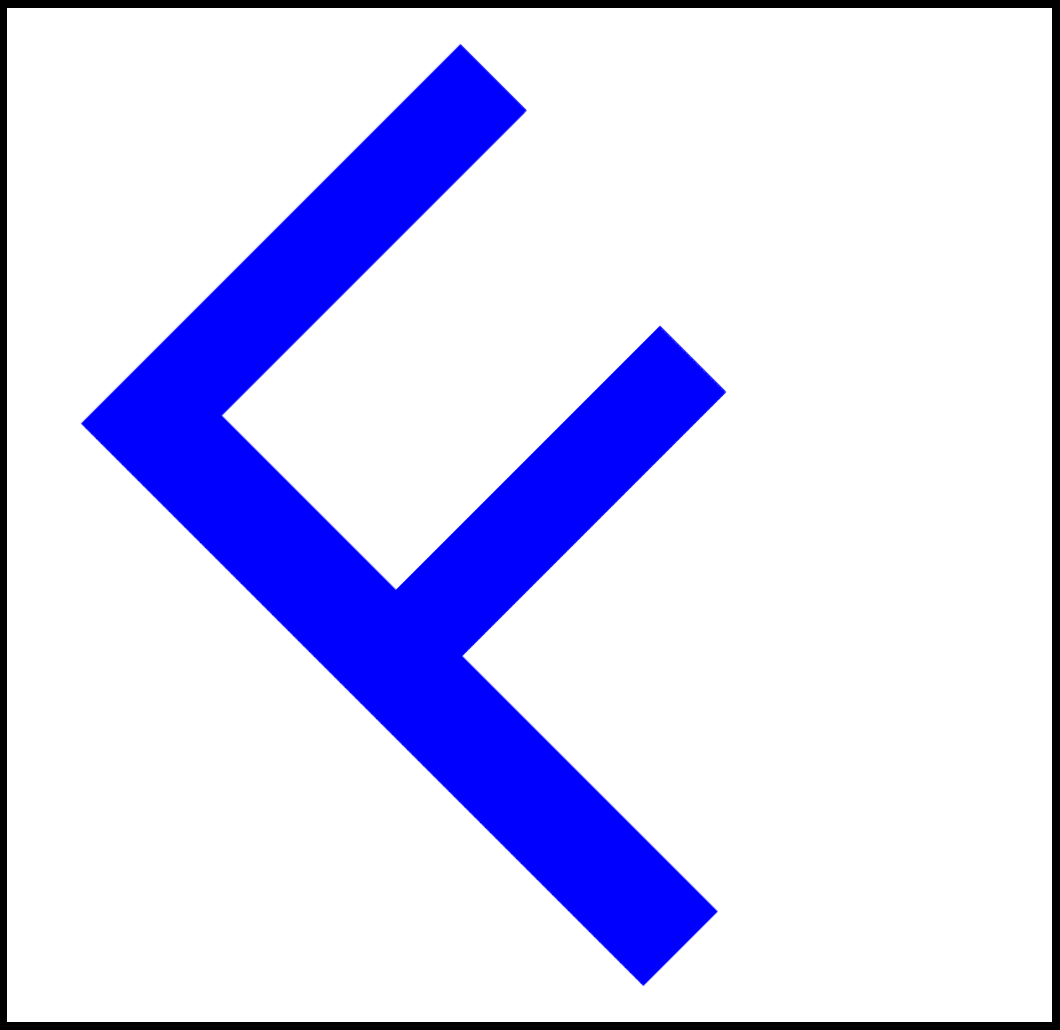
Tile rotation=-45°. |
Tile rotation=-20°. |
Original tile. |

Tile rotation=20°. |

Tile rotation=45°. |
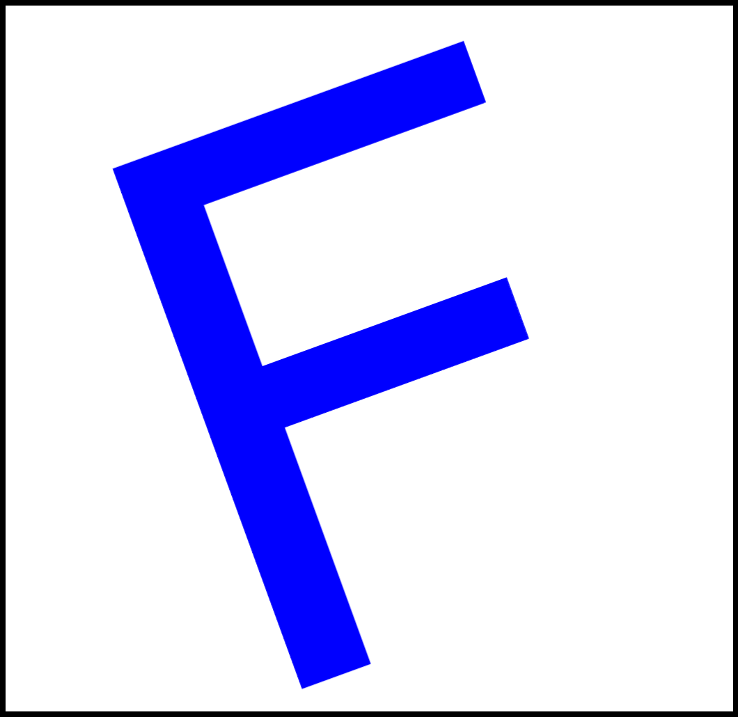
In Classify Object and Segment Instances, for an image with the feature "F" and given augmentation values, samples as below can be added to the training set.
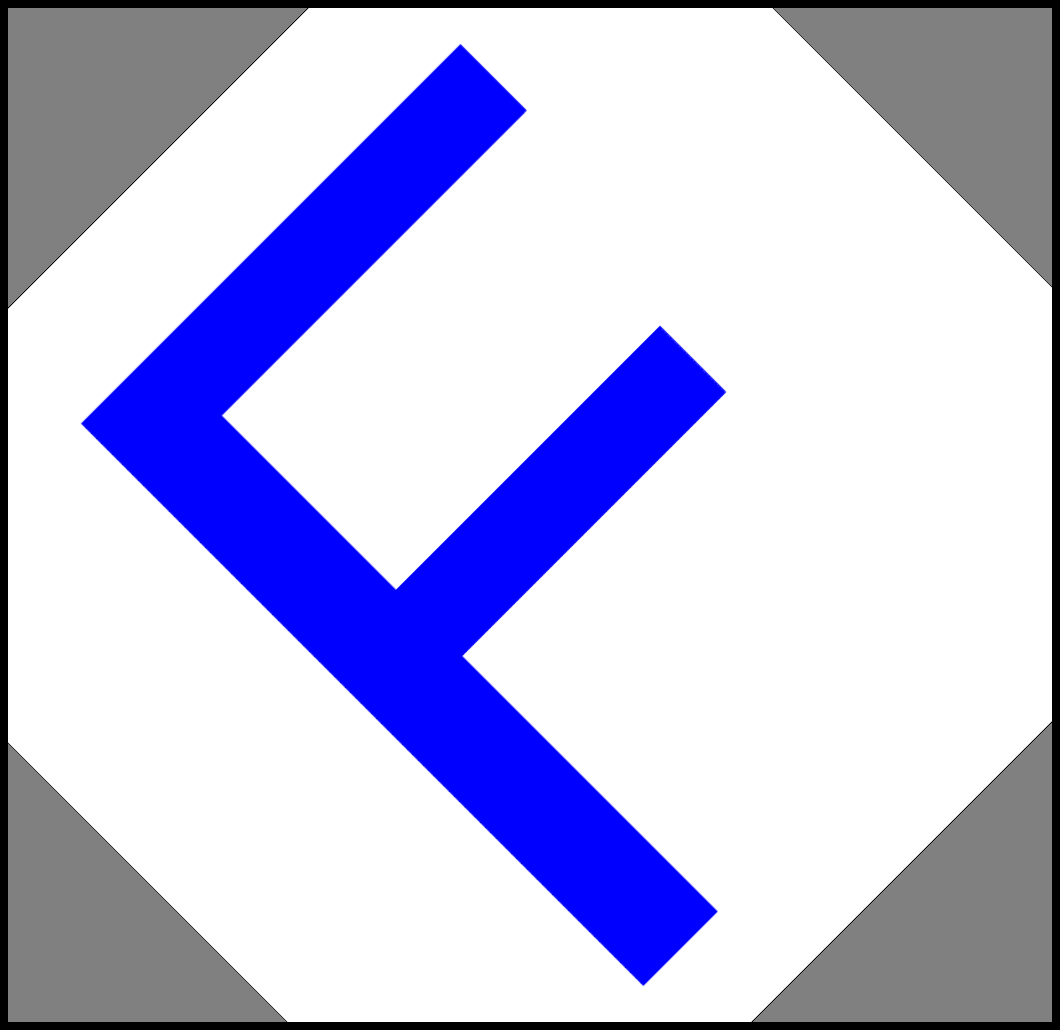
Image rotation=-45°. |

Image rotation=-20°. |
Original image. |

Image rotation=20°. |

Image rotation=45°. |
|
No flips. |
Up-Down flip. |
Left-Right flip. |
Both flips. |
In Locate Points, for a tile with the feature "F" and given augmentation values, samples as below can be added to the training set.
|
Tile translation x=20%, y=20%. |
Original tile. |
Tile translation x=-20%, y=-20%. |

Resize=50%. |
Original image. |
Resize=150%. |
In Detect Features, Locate Points and Detect Anomalies, for a tile with the feature "F" and given augmentation values, samples as below can be added to the training set.
Horizontal Shear=-30. |
Original tile. |
Horizontal Shear=30. |
In Classify Object and Segment Instances, for an image with the feature "F" and given augmentation values, samples as below can be added to the training set.

Horizontal Shear=-30. |
Original image. |

Horizontal Shear=30. |
In Detect Features, Locate Points, and Detect Anomalies, for a tile with the feature "F" and given augmentation values, samples as below can be added to the training set.
Vertical Shear=-30. |
Original tile. |
Vertical Shear=30. |
In Classify Object and Segment Instances, for an image with the feature "F" and given augmentation values, samples as below can be added to the training set.
Vertical Shear=-30. |
Original image. |
Vertical Shear=30. |
Warning: the choice of augmentation options depends only on the task we want to solve. Sometimes they might be harmful for quality of a solution. For a simple example, the Rotation should not be enabled if rotations are not expected in a production environment. Enabling augmentations also increases the network training time (but does not affect execution time!)
2. Anomaly Detection
FabImage Deep Learning provides three ways of defect detection:
- FisFilter_DL_DetectAnomalies1
- FisFilter_DL_DetectAnomalies2 Golden Template
- FisFilter_DL_DetectAnomalies2 Similarity-Based
The FisFilter_DL_DetectAnomalies1 (reconstructive approach) uses deep neural networks to remove defects from the input image by reconstructing the affected regions.
It is used to analyze images in fragments of size determined by the Feature Size parameter.
This approach is based on reconstructing an image without defects and then comparing it with the original one.
It filters out all patterns smaller than Feature Size that were not present in the training set.
The FisFilter_DL_DetectAnomalies2 Golden Template is an appropriate method for positioned objects with complex details. The tool divides the images into regions and creates a separate model for each region. The tool has the Texture Mode dedicated for texture defects detection. It can be used for plain surfaces or the ones with a simple pattern.
The FisFilter_DL_DetectAnomalies2 Similarity-Based is a good general-purpose technique that can handle detailed as well as simple datasets. The tool operates by first assembling a collection of normal features during training and then by comparing observed image segments against this collection during inference to assess normality.
To sum up, while choosing the tool for anomaly detection, first check the Similarity-Based approach. If the model isn't producing sufficiently accurate defect localizations, please try the Golden Template approach. If the object is complex and its position is unstable, please check the FisFilter_DL_DetectAnomalies1 approach.
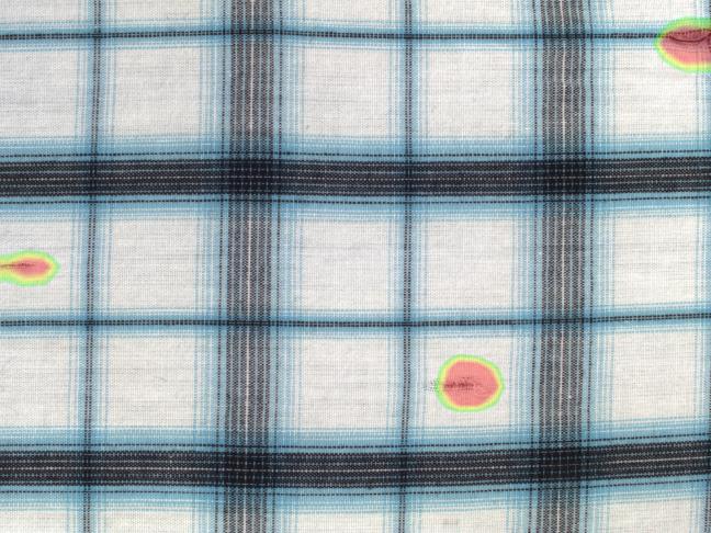
An example of textile defect detection using the FisFilter_DL_DetectAnomalies2.
Parameters
-
Feature Size is related to FisFilter_DL_DetectAnomalies1 approach.
It corresponds to the expected defect size and it is the most significant one in terms of both quality and speed of inspection.
It is represented by a green square in the Image window of the Editor. The common denominator of all fragment based approaches is that the Feature Size should be adjusted so that it contains common defects with some margin.
For FisFilter_DL_DetectAnomalies1 large Feature Size will cause small defects to be ignored, however the inference time will be shortened considerably. Heatmap precision will also be lowered. Consider using Downscale parameter instead of increasing the Feature Size. - Sampling Density is related to the FisFilter_DL_DetectAnomalies1 approach. It controls the spatial resolution of both training and inspection. The higher the density the more precise results but longer computational time.
- Max Translation is related to the FisFilter_DL_DetectAnomalies2 Golden Template approach. It is the maximal position change tolerance. If the parameter increases, the working area of a small model enlarges and the number of the created small models decreases.
- Model Complexity (or just Complexity) is related to the FisFilter_DL_DetectAnomalies2 approach. Greater value may improve model effectiveness, especially for complex objects, at the expense of memory usage and interference time.
Metrics
Measuring accuracy of anomaly detection tools is a challenging task. The most straightforward approach is to calculate the Recall/Precision/F1 measures for the whole images (classified as GOOD or BAD, without looking at the locations of the anomalies). Unfortunately, such an approach is not very reliable due to several reasons, including: (1) when we have a limited number of test images (like 20), the scores will vary a lot (like Δ=5%) when just one case changes; (2) very frequently the tools we test will find random false anomalies, but will not find the right ones - and still will get high scores as the image as a whole is considered correctly classified. Thus, it may be tempting to use annotated anomaly regions and calculate the per-pixel scores. However, this would be too fine-grained. For anomaly detection tasks we do not expect the tools to be necessarily very accurate in terms of the location of defects. Individual pixels do not matter much. Instead, we expect that the anomalies are detected "more or less" at the right locations. As a matter of fact, some tools which are not very accurate in general (especially those based on auto-encoders) will produce relatively accurate outlines for the anomalies they find, while the methods based on one-class classification will usually perform better in general, but the outlines they produce will be blurred, too thin or too thick.
For these reasons, we introduced an intermediate approach to calculation of Recall. Instead of using the per-image or the per-pixel methods, we use a per-region one. Here is how we calculate Recall:
- For each anomaly region we check if there is any single pixel in the heatmap above the threshold. If it is, we increase TP (the number of True Positives) by one. Otherwise, we increase FN (the number of False Negatives) by one.
- Then we use the formula: $${Recall = \frac{TP}{TP + FN} }$$
The above method works for Recall, but cannot be directly applied to the calculation of Precision. Thus, for Precision we use a per-pixel approach, but it also comes with its own difficulties. First issue is that we often find ourselves having a lot of GOOD samples and a very limited set of BAD testing cases. This means unbalanced testing data, which in turn means that the Precision metric is highly affected with the overwhelming quantity of GOOD samples. The more GOOD samples we have (at the same amount of BAD samples), the lower Precision will be. It may be actually very low, often not reflecting the true performance of the tool. For that reason, we need to incorporate balancing into our metrics.
A second issue with Precision in real-world projects is that False Positives tend to naturally occur within BAD images, outside of the marked anomaly regions. This happens for several reasons, but is repeatable among different projects. Sometimes if there is a defect, it often means that something was broken and other parts of the object may be slightly affected too, sometimes in a visible way, sometimes with a level of ambiguity. And quite often the objects under inspection simply get affected by the process of artificially introducing defects (like someone is touching a piece of fabric and accidentally causes wrinkles that would normally not occur). For this reason, we calculate the per-pixel False Negatives only on GOOD images.
The complete procedure for calculation of Precision is:
- We calculate the average pp_TP (the number of per-pixel True Positives) across all BAD testing samples.
- We calculate the average pp_FP (the number of per-pixel False Positives) across all GOOD testing samples.
- Then we use the formula: $${Precision=\frac{\overline{pp\underline{}TP} }{\overline{pp\underline{}TP} + \overline{pp\underline{}FP} } }$$
Finally we calculate the F1 score in the standard way, for practical reasons neglecting the fact that the Recall and Precision values that we unify were calculated in different ways. We believe that this metric is best for practical applications.
Model Usage
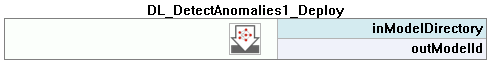
In Detect Anomalies 1 variant, a model should be loaded with FisFilter_DL_DetectAnomalies1_Deploy prior to executing it with FisFilter_DL_DetectAnomalies1. Alternatively, the model can be loaded directly by FisFilter_DL_DetectAnomalies1 filter, but it will then require time-consuming initialization in the first program iteration.
In Detect Anomalies 2 variant, a model should be loaded with FisFilter_DL_DetectAnomalies2_Deploy prior to executing it with FisFilter_DL_DetectAnomalies2. Alternatively, model can be loaded directly by FisFilter_DL_DetectAnomalies2 filter, but it will then require time-consuming initialization in the first program iteration.

Running FabImage Deep Learning Service simultaneously with these filters is discouraged as it may result in degraded performance or errors.
3. Feature Detection (segmentation)
This technique is used to detect pixel-wise regions corresponding to defects or – in a general sense – to any image features. A feature here may be also something like the roads on a satellite image or an object part with a characteristic surface pattern. Sometimes it is also called pixel labeling as it assigns a class label to each pixel, but it does not separate instances of objects.
Training Data
Images used for training can be of different sizes and can have different ROIs defined. However, it is important to ensure that the scale and the characteristics of the features are consistent with that of the production environment.
Each and every feature should be marked on all training images, or the ROI should be limited to include only marked defects. Incompletely or inconsistently marked features are one of the main reasons of poor accuracy. REMEMBER: If you leave even a single piece of some feature not marked, it will be used as a negative sample and this will highly confuse the training process!
The marking precision should be adjusted to the application requirements. The more precise marking the better accuracy in the production environment. While marking with low precision it is better to mark features with some excess margin.
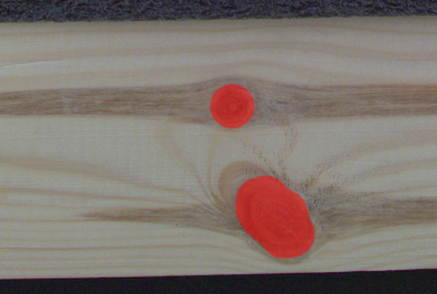
An example of wood knots marked with low precision. |
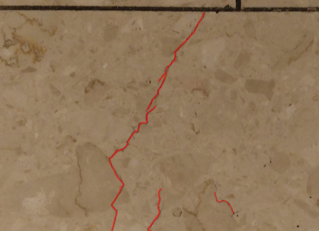
An example of tile cracks marked with high precision. |
Multiple classes of features
It is possible to detect many classes of features separately using one model. For example, road and building like in the image below. Different features may overlap but it is usually not recommended. Also, it is not recommended to define more than a few different classes in a single model. On the other hand, if there are two features that may be mutually confusing (e.g. roads and rivers), it is recommended to have separate classes for them and mark them, even if one of the classes is not really needed in the results. Having the confusing feature clearly marked (and not just left as the background), the neural network will focus better on avoiding misclassification.
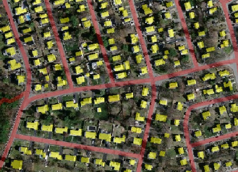
An example of marking two different classes (red roads and yellow buildings) in the one image.
Patch Size
Detect Features is an end-to-end segmentation tool which works best when analysing an image in a medium-sized square window. The size of this window is defined by the Patch Size parameter. It should be not too small, and not too big. Typically much bigger than the size (width or diameter) of the feature itself, but much less than the entire image. In a typical scenario the value of 96 or 128 works quite well.
Performance Tip 1: a larger Patch Size increases the training time and requires more GPU memory and more training samples to operate effectively. When Patch Size exceeds 128 pixels and still looks too small, it is worth considering the Downsample option.
Performance Tip 2: if the execution time is not satisfying you can set the inOverlap filter input to False. It should speed up the inspection by 10-30% at the expense of less precise results.
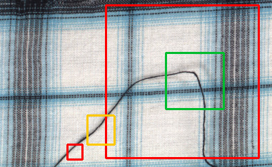
Examples of Patch Size: too large or too small (red), maybe acceptable (yellow) and good (green). Remember that this is just an example and may vary in other cases.
Model Usage
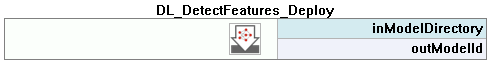
A model should be loaded with FisFilter_DL_DetectFeatures_Deploy filter before using FisFilter_DL_DetectFeatures filter to perform segmentation of features. Alternatively, the model can be loaded directly by FisFilter_DL_DetectFeatures filter, but it will result in a much longer time of the first iteration.
Running FabImage Deep Learning Service simultaneously with these filters is discouraged as it may result in degraded performance or errors.
Parameters:
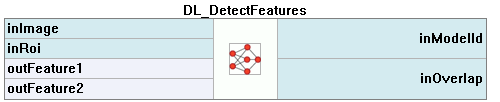
- To limit the area of image analysis you can use inRoi input.
- To shorten feature segmentation process you can disable inOverlap option. However, in most cases, it decreases segmentation quality.
- Feature segmentation results are passed in a form of bitmaps to outHeatmaps output as an array and outFeature1, outFeature2, outFeature3 and outFeature4 as separate images.
4. Object Classification
This technique is used to identify the class of an object within an image or within a specified region.
The Principle of Operation
During the training phase, the object classification tool learns representation of user defined classes. The model uses generalized knowledge gained from samples provided for training, and aims to obtain good separation between the classes.
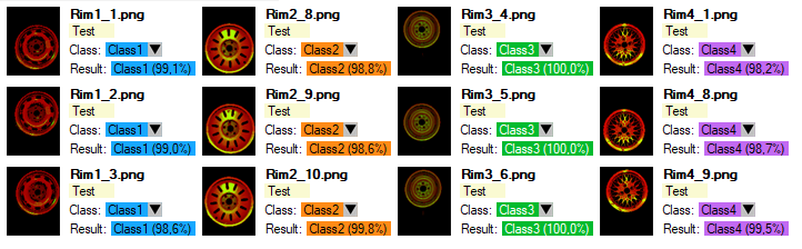
Result of classification after training.
After a training process is completed, the user is presented with a confusion matrix. It indicates how well the model separated the user defined classes. It simplifies identification of model accuracy, especially when a large number of samples has been used.
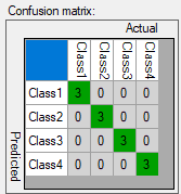
Confusion matrix presents correct (diagonal) and incorrect assignment of samples to the user defined classes.
Training Parameters
In addition to the default training parameters (list of parameters available for all Deep Learning algorithms), the FisFilter_DL_ClassifyObject tool provides a Detail Level parameter which enables control over the level of detail needed for a particular classification task. For majority of cases the default value of 1 is appropriate, but if images of different classes are distinguishable only by small features (e.g. granular materials like flour and salt), increasing value of this parameter may improve classification results.
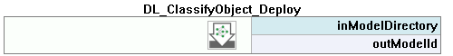
Model Usage
A model should be loaded with FisFilter_DL_ClassifyObject_Deploy filter before using FisFilter_DL_ClassifyObject filter to perform classification. Alternatively, model can be loaded directly by FisFilter_DL_ClassifyObject filter, but it will result in a much longer time of the first iteration.
Running FabImage Deep Learning Service simultaneously with these filters is discouraged as it may result in degraded performance or errors.
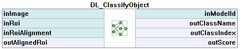
Parameters:
- To limit the area of image analysis you can use inRoi input.
- Classification results are passed to outClassName and outClassIndex outputs.
- The score value outScore indicates the confidence of classification.
5. Instance Segmentation (deprecated)
The Instance Segmentation model is trainable in 5.3 and older versions only. In more recent releases, models trained in 5.3 and older versions can only be inferred.This technique is used to locate, segment and classify one or multiple objects within an image. The result of this technique are lists with elements describing detected objects – their bounding boxes, masks (segmented regions), class IDs, names and membership probabilities.
Note that in contrary to feature detection technique, instance segmentation detects individual objects and may be able to separate them even if they touch or overlap. On the other hand, instance segmentation is not an appropriate tool for detecting features like scratches or edges which may possibly have no object-like boundaries.
Original image. |
Visualized instance segmentation results. |
Training Data
The training phase requires the user to draw regions corresponding to objects on an image and assign them to classes.
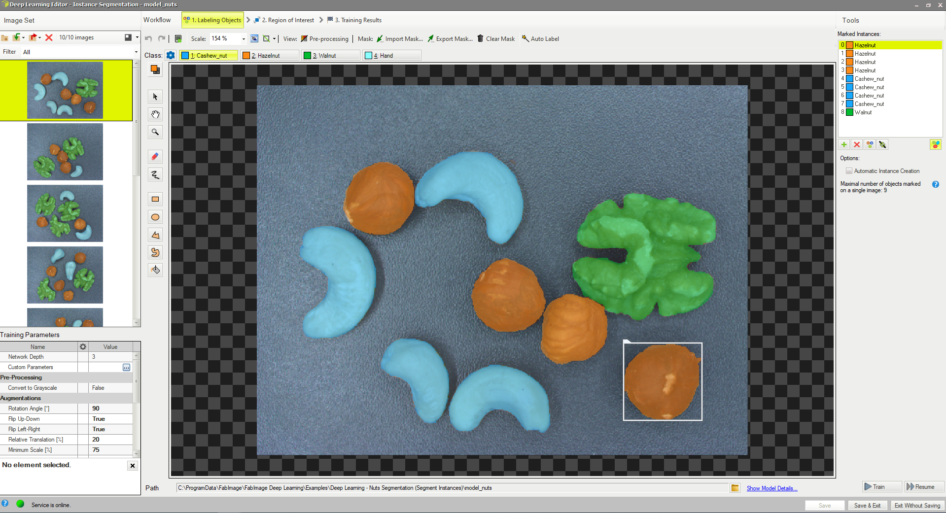
Editor for marking objects.
Training Parameters
Instance segmentation training adapts to the data provided by the user and does not require any additional training parameters besides the default ones.
Model Usage
A model should be loaded with FisFilter_DL_SegmentInstances_Deploy_Deprecated filter before using FisFilter_DL_SegmentInstances_Deprecated filter to perform classification. Alternatively, model can be loaded directly by FisFilter_DL_SegmentInstances_Deprecated filter, but it will result in a much longer time of the first iteration.
Running FabImage Deep Learning Service simultaneously with these filters is discouraged as it may result in degraded performance or errors.
Parameters:
- To limit the area of image analysis you can use inRoi input.
- To set minimum detection score inMinDetectionScore parameter can be used.
- Maximum number of detected objects on a single image can be set with inMaxObjectsCount parameter. By default it is equal to the maximum number of objects in the training data.
- Results describing detected objects are passed to following outputs:
- bounding boxes: outBoundingBoxes,
- class IDs: outClassIds,
- class names: outClassNames,
- classification scores: outScores,
- masks: outMasks.
6. Point Location
This technique is used to precisely locate and classify key points, characteristic parts and small objects within an image. The result of this technique is a list of predicted point locations with corresponding class predictions and confidence scores.
When to use point location instead of instance segmentation:
- precise location of key points and distinctive regions with no strict boundaries,
- location and classification of objects (possibly very small) when their segmentation masks and bounding boxes are not needed (e.g. in object counting).
When to use point location instead of feature detection:
- coordinates of key points, centroids of characteristic regions, objects etc. are needed.
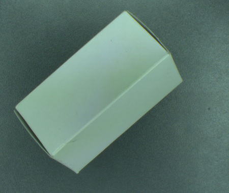
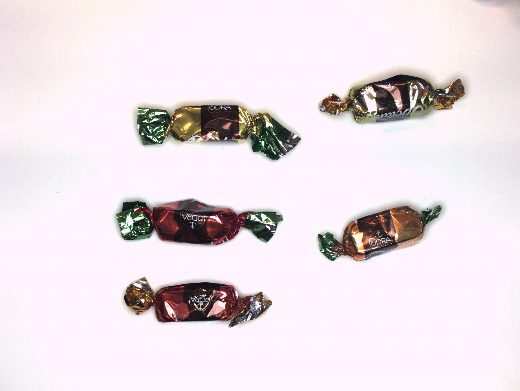
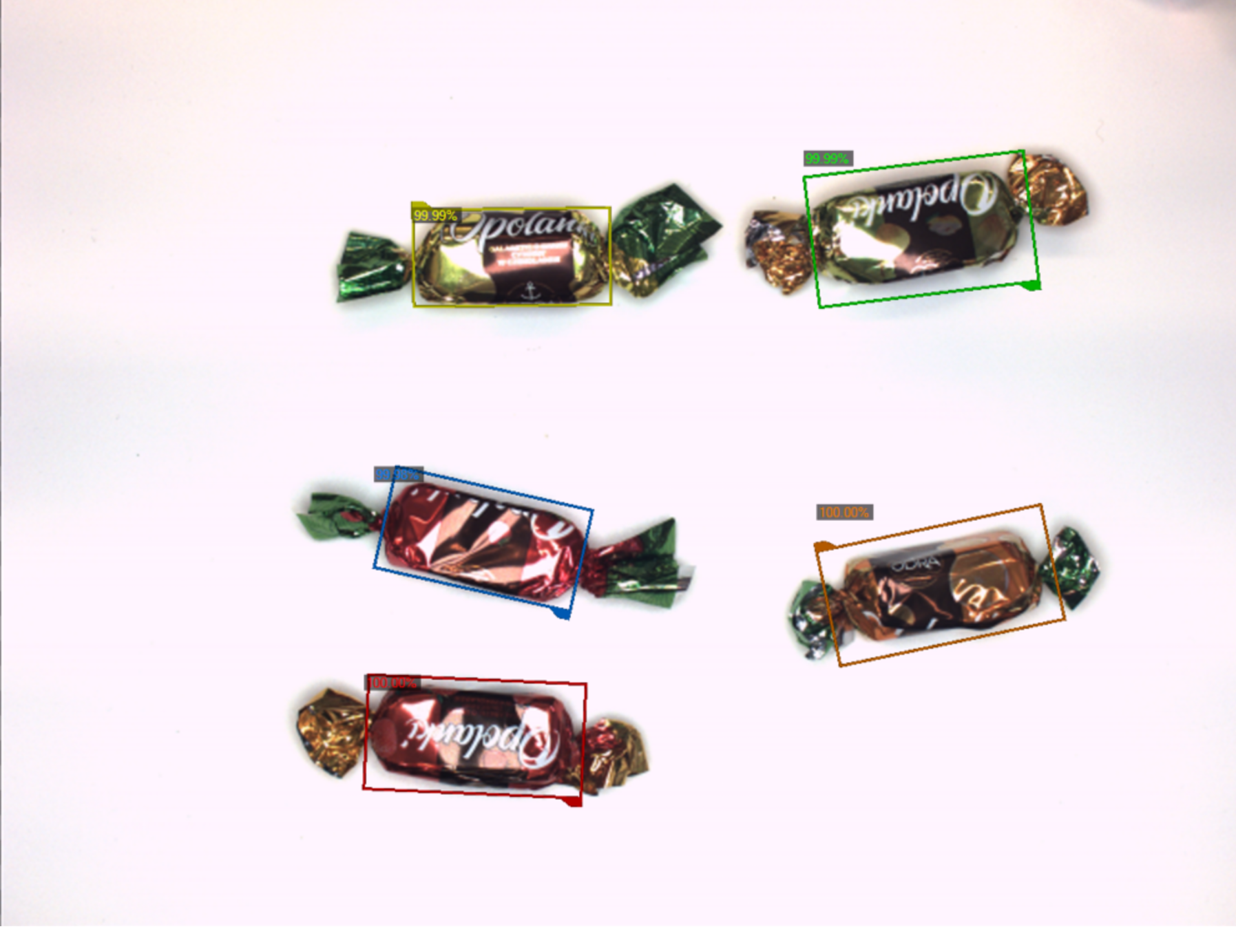
Original image. |
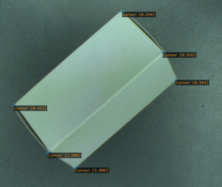
Visualized point location results. |
Training Data
The training phase requires the user to mark points of appropriate classes on the training images.
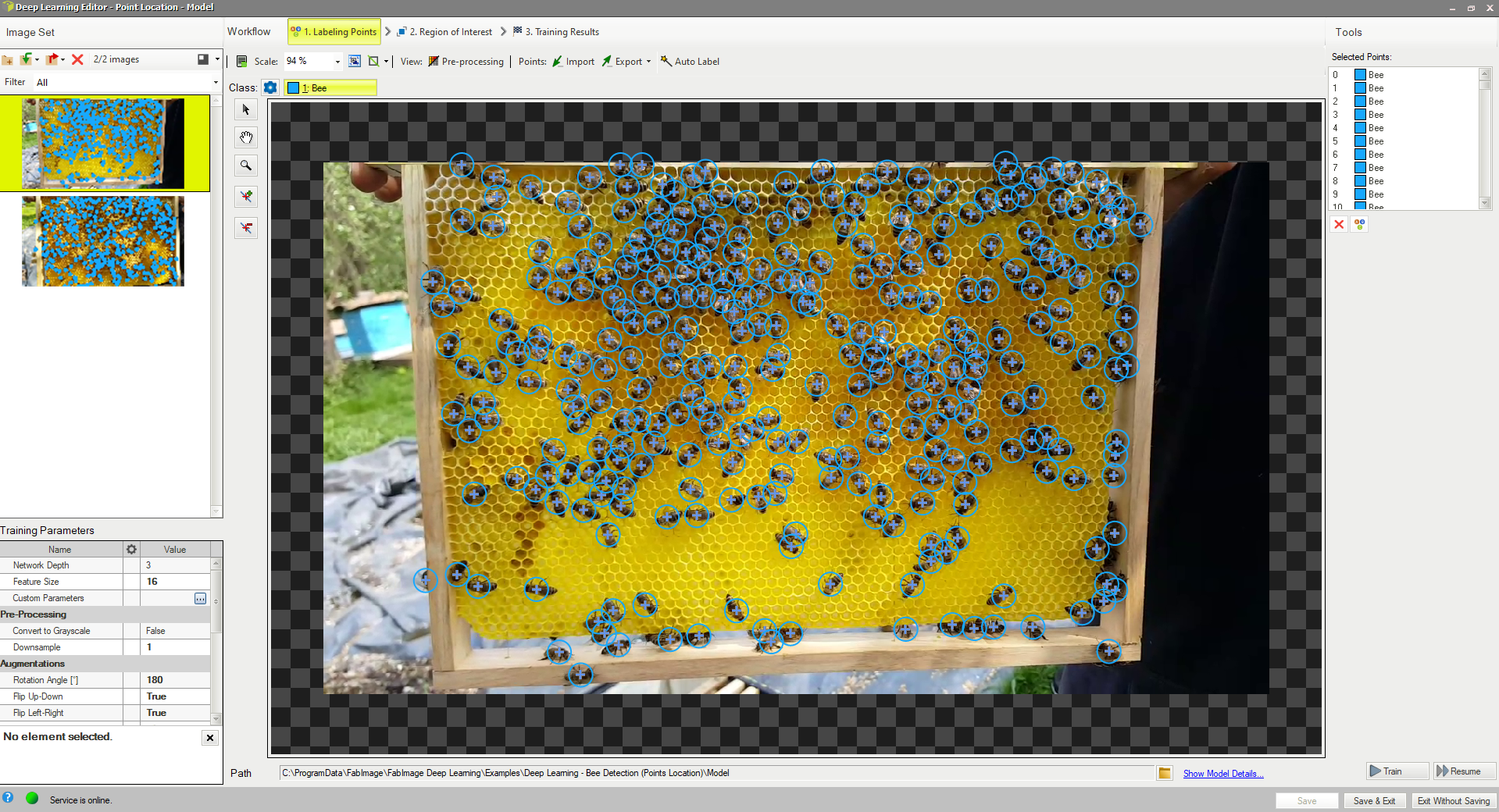
Editor for marking points.
Feature Size
In the case of the Point Location tool, the Feature Size parameter corresponds to the size of an object or characteristic part. If images contain objects of different scales, it is recommended to use a Feature Size slightly larger than the average object size, although it may require experimenting with different values to achieve the best possible results.
Performance tip: a larger feature size increases the training time and needs more memory and training samples to operate effectively. When feature size exceeds 64 pixels and still looks too small, it is worth considering the Downsample option.
Model Usage
A model should be loaded with FisFilter_DL_LocatePoints_Deploy filter before using FisFilter_DL_LocatePoints filter to perform point location and classification. Alternatively, model can be loaded directly by FisFilter_DL_LocatePoints filter, but it will result in a much longer time of the first iteration.
Running FabImage Deep Learning Service simultaneously with these filters is discouraged as it may result in degraded performance or errors.
Parameters:
- To limit the area of image analysis you can use inRoi input.
- To set minimum detection score inMinDetectionScore parameter can be used.
- inMinDistanceRatio parameter can be used to set minimum distance between two points to be considered as different. The distance is computed as MinDistanceRatio * FeatureSize. If the value is not enabled, the minimum distance is based on the training data.
- To increase detection speed but with potentially slightly worse precision inOverlap can be set to False.
- Results describing detected points are passed to following outputs:
- point coordinates: outLocations,
- class IDs: outClassIds,
- class names: outClassNames,
- classification scores: outScores.
7. Locating objects
This technique is used to locate and classify one or multiple objects within an image. The result of this technique is a list of rectangles bounding the predicted objects with corresponding class predictions and confidence scores.
The tool returns the rectangle region containing the predicted objects and showing their approximate location and orientation, but it doesn't return the precise position of the key points of the object or the segmented region. It is an intermediate solution between the Point Location and the Instance Segmentation.
Original image. |
Visualized object location results. |
Training Data
The training phase requires the user to mark rectangles bounding objects of appropriate classes on the training images.
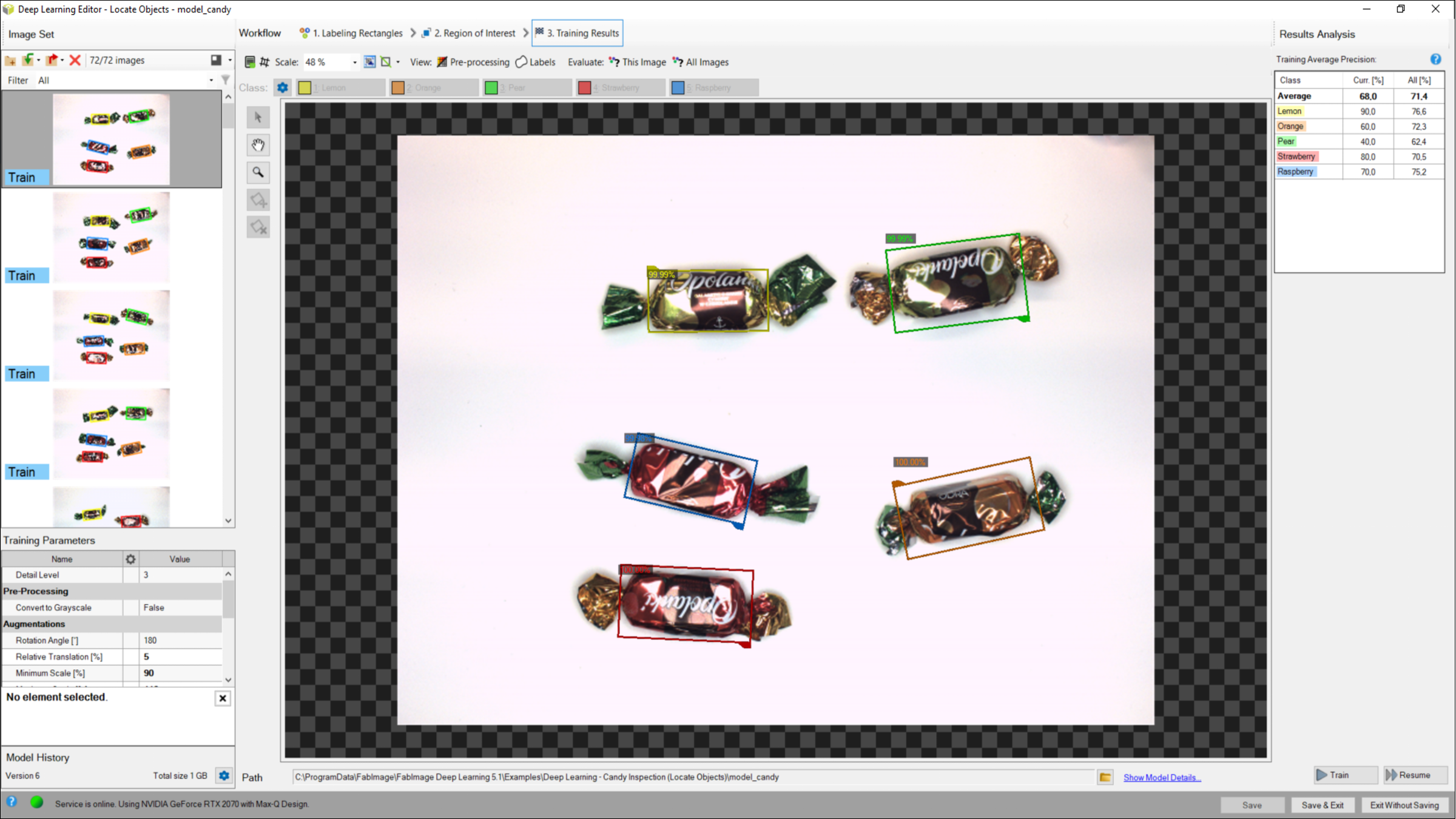
Editor for marking objects.
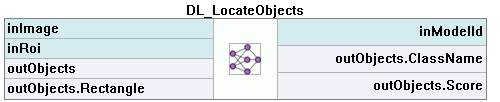
Model Usage
A model should be loaded with FisFilter_DL_LocateObjects_Deploy filter before using FisFilter_DL_LocateObjects filter to perform object location and classification. Alternatively, model can be loaded directly by FisFilter_DL_LocateObjects filter, but it will result in a much longer time of the first iteration.

Running FabImage Deep Learning Service simultaneously with these filters is discouraged as it may result in degraded performance or errors.
Parameters:
- To limit the area of image analysis you can use inRoi input.
- To set minimum detection score inMinDetectionScore parameter can be used.
- Results describing detected objects are passed to the object output: outObjects.
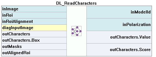
8. Reading Characters
This technique is used to locate and recognize characters within an image. The result is a list of found characters.
This tool uses a pretrained model and cannot be trained.
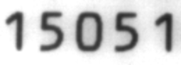
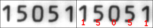
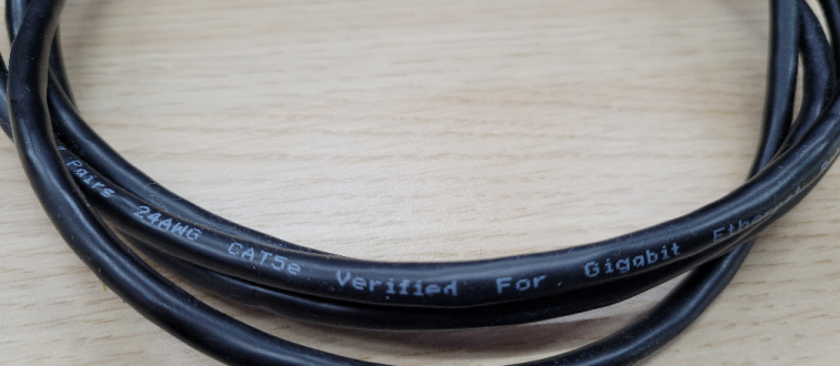
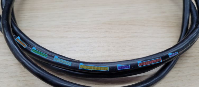
Original image. |

Visualized results of the OCR tool. |
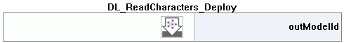
Model Usage
A model should be loaded with the FisFilter_DL_ReadCharacters_Deploy filter before using the FisFilter_DL_ReadCharacters filter to perform recognition. Alternatively, a model can be loaded directly by the FisFilter_DL_ReadCharacters filter, but it may result in a longer time of the first iteration.
Running the FabImage Deep Learning Service simultaneously with these filters is discouraged as it may result in degraded performance or errors.
Parameters:
- To limit the area of the image analysis and/or to set a text orientation you can use the inRoi input.
- You can set one of the available pretrained model types in the FisFilter_DL_ReadCharacters_Deploy filter using the inPretrainedModelType input or, in the FisFilter_DL_ReadCharacters filter, using the inModelID/PretrainedModel input. Differences between the various model types are elaborated upon here.
- The average size (in pixels) of characters in the analysed area should be set with the inCharHeight parameter. Here you can learn more about the relation between the inCharRange input value and the type of model that you selected.
- To improve the detection/recognition accuracy for a font with exceptionally thin or wide contours you can use theinWidthScale input. To some extent, it may also help in case of characters positioned very close to each other.
- To filter false positive results near true characters use inCharSpacing parameter.
- To limit or increase the set of recognized characters (e.g. to exclude digits or to include punctuation marks) use the inCharRange parameter.
- To filter results by polarity and contrast use inPolarization and inContrastThreshold parameters.
- To remove results at the edge of ROI inRemoveBoundaryCharacters parameter.
- To get string by connection outCharacters
- To match known inPattern use grammar rules
9. Locating Text
This technique is used to locate text within an image. The result is an array of found located rectangles.
This tool uses a pretrained model and cannot be trained.
Original image. |
Visualized text location results, with orientation marked at origin. |
Model Usage
A model should be loaded with the FisFilter_DL_LocateText_Deploy filter before using the FisFilter_DL_LocateText filter to perform recognition. Alternatively, model can be loaded directly by the FisFilter_DL_LocateText filter, but it may result in a longer time of the first iteration.
Running FabImage Deep Learning Service simultaneously with these filters is discouraged as it may result in degraded performance or errors.
Parameters:
- To limit the area of image analysis you can use the inRoi input.
- You can set one of the available pretrained model types in the FisFilter_DL_LocateText filter using the inModelID/PretrainedModel input. Differences between the various model types are elaborated upon here.
- The average size (in pixels) of characters in the analysed area should be set with the inCharHeight parameter. Here you can learn more about the relation between the inCharRange input value and the type of model that you selected.
- To improve the detection accuracy for a font with exceptionally thin or wide contours you can use the inWidthScale input. To some extent, it may also help in case of characters positioned very close to each other.
- To set the minimum area value threshold for detection, inMinTextArea parameter can be used.
10. Troubleshooting
Below you will find a list of most common problems.
1. Network overfitting
A situation when a network loses its ability to generalize over available problems and focuses only on training data.
Symptoms: during training, the loss graph starts rising, the validation graph stops at one level and training graph continues to rise. Defects on training images are marked very precisely, but defects on new images are marked poorly.
A graph characteristic for network overfitting.
Causes:
- The number of test samples is too small.
- Training time is too long.
Possible solutions:
- Provide more real samples of different objects.
- Use more augmentations.
- Reduce Network Depth.
2. Susceptibility to changes in lighting conditions
Symptoms: network is not able to process images properly when even minor changes in lighting occur.
Causes:
- Samples with variable lighting were not provided.
Solution:
- Provide more samples with variable lighting.
- Enable "Luminance" option for automatic lighting augmentation.
3. No progress in network training
Symptoms ― even though the training time is optimal, there is no visible training progress.
Training progress with contradictory samples.
Causes:
- The number of samples is too small or the samples are not variable enough.
- Image contrast is too small.
- The chosen network architecture is too small.
- There is contradiction in defect masks.
Solution:
- Modify lighting to expose defects.
- Remove contradictions in defect masks.
Tip: Remember to mark all defects of a given type on the input images or remove images with unmarked defects. Marking only a part of defects of a given type may negatively influence the network learning process.
4. Training/sample evaluation is very slow
Symptoms ― training or sample evaluation takes a lot of time.
Causes:
- Resolution of the provided input images is too high.
- Fragments that cannot possibly contain defects are also analyzed.
Solution:
- Enable "Downsample" option to reduce the image resolution.
- Limit ROI for sample evaluation.
- Use lower Network Depth
See Also
- Deep Learning training API documentation - instruction how to perform training of Deep Learning models (5.3 and older version only).
| Previous: Golden Template | Next: Function Reference |